How to Nest, or Group, Rows in Excel

If your spreadsheet is complex and chock-full of data, it might help to learn how to group, or nest, your rows in Excel for easier visibility.
Dealing with a spreadsheet that’s chock-full of data and percentages can feel like you’re lost in a digital jungle of rows. It’s like trying to find that one tree in a forest — pretty tedious, right? But don’t worry, Excel comes to the rescue like a superhero! We’ve got one more tip on how to get the most out of Excel. Let’s dive into how you can tame this wild beast by learning how to nest or group rows in Excel. It’s like giving your data a cozy little home where everything’s easy to find!
Getting That Mass of Data Under Control
When you find yourself battling that digital jungle, you’ll find that grouping rows into particular chunks helps keep a handle on all that data. Once you’ve learned how to nest rows in Excel, you can organize your data such that you can easily collapse the rows you don’t want to see.
How to Use Excel’s Outline Feature to Group, or Nest, Rows
To group rows together, just follow these steps.
- Select the rows you want to group. You can click the first row and then hold the Shift key when you click the last row. Or, you can click and drag the row headings to select them.
- In the Ribbon selections, click Data.

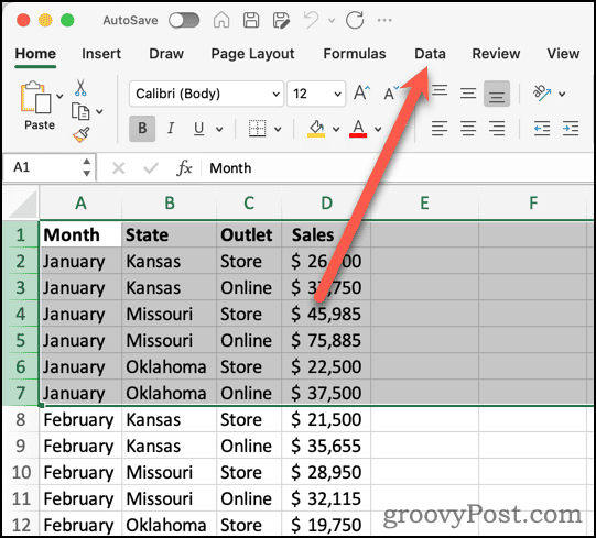
- Click the Group button.


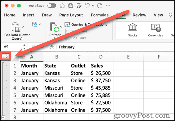
- Excel will add a connection line and minus sign for the selected rows. It also adds level buttons (1, 2, etc.) for the different levels of your outline.

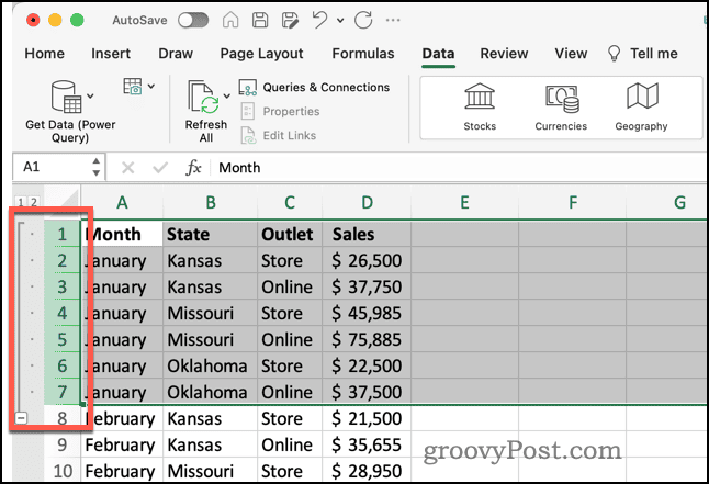
Adding More Row Groups to Your Excel Spreadsheet
If you want to group additional sets of rows, you can. It’s important to note, though, that you need an empty row between the last row of one group and the beginning of another. If there isn’t an empty row, Excel will add the new rows to the existing group.
This sort of outlining and organization can definitely make it easier to work with your data. For example, if you need to create a pie chart of just a segment of your information, it becomes much easier to see exactly the rows you want to work with and not the rest of the data.
Collapsing or Expanding Groups of Rows
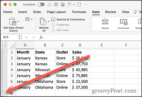
Now, you can tame your jungle of rows considerably, using the groups’ minus signs to collapse groups. This way, you can easily hide data for a less cluttered view of what you need to work with.
- When you want to collapse a group of rows, click the Minus sign (-) to hide the group.

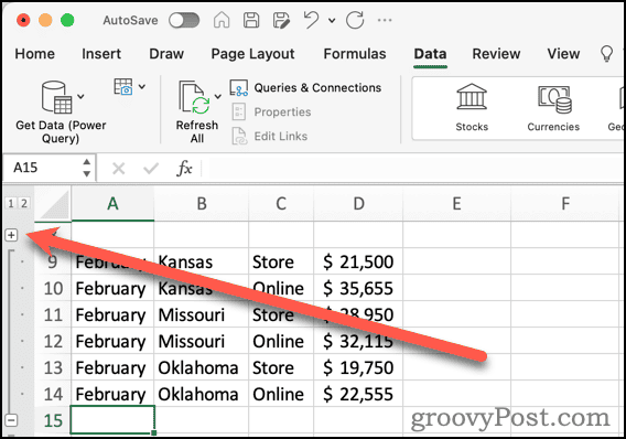
- To see the rows again, click the Plus sign (+).

- You can also use the 1 at the top of the row headings to collapse your group. The 2 button expands the group.

Adding Subgroups to Your Data
Maybe you want to organize your rows even further. You can create subgroups within a group of rows.
- Select the rows you want to include in the subgroup.
- Click Group.
- A nested subgroup appears, along with a new button labeled 3.
- Clicking 2 collapses any subgroups. Click 3 to expand the subgroups once again.
Using Excel’s Subtotal Feature to Nest Rows
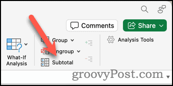
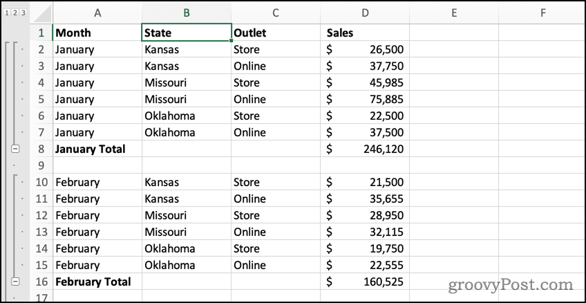
If you know you need subtotals of one or more columns in your groups, Excel has a similar feature to help organize the outline of rows. Located in the same area of the Data ribbon as the Group and Ungroup buttons, it’s called Subtotal.
How to Nest or Group Rows Using Subtotal in Excel
- Choose the rows you want organized into groups.
- Click Subtotal.

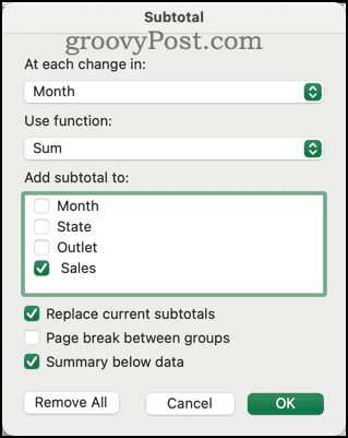
- The next dialog allows you to adjust how Excel organizes your rows into groups and for which columns it calculates subtotals.

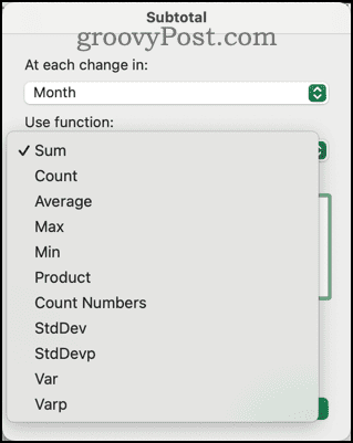
- You can also choose a function like COUNT instead of SUM to use within your subtotals.

- Click OK to finalize your settings and create your groups and subtotal fields.

Working Smarter With Your Data in Excel
By applying smart groupings of your rows in Excel, you can tame the mass of data in your spreadsheet. This can make it much easier to view and edit your information without endless scrolling and searching.
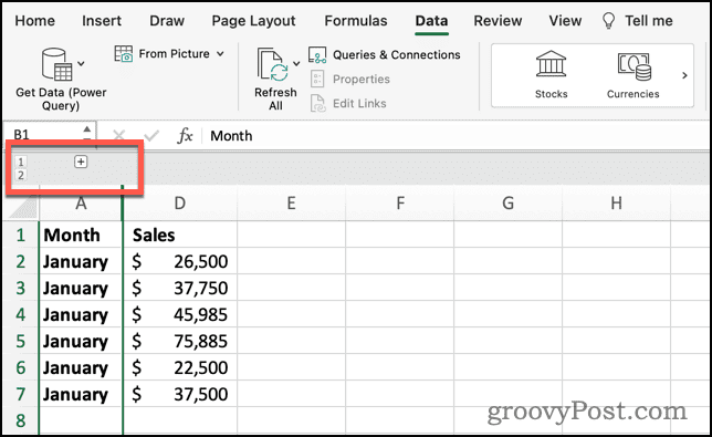
As a final note, all of the previous steps can also be used to group or nest columns rather than rows. Just select the columns instead, and Excel will handle the outlining for you.

Leave a Reply
Leave a Reply


