How to Freeze, Hide, and Group Columns and Rows in Excel

Manage your columns and rows in Excel to make your data easier to view or enter. Learn to freeze, hide, and group columns and rows with this how-to.
When you work with a spreadsheet application like Microsoft Excel, it’s important to know how to manage columns and rows. We’ve shown you essential Excel tips like adding and removing them as well as how to convert rows to columns. But there’s more!
You can freeze, hide, and group the columns and rows in Excel to give you a better view of your data. Here, we’ll show you how to do all three.
Freeze and Unfreeze Columns and Rows in Excel
If you have a lengthy spreadsheet or one that covers many columns, freezing can help. You can freeze the top row or the first column to keep it in view when you scroll. This is super handy for heavy data entry tasks.
In your Excel spreadsheet, select the View tab.
On Windows, click Freeze Panes in the ribbon and choose Freeze Top Row or Freeze First Column. You can also enable both if needed.
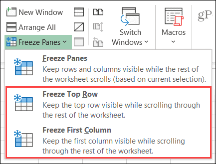

On Mac, you have buttons for each Freeze option. So just click Freeze Top Row or Freeze First Column, or both if you like.


You’ll notice a thin border appear for the row or column you freeze. And when you scroll down or sideways, the column or row will remain in view.
To unfreeze, click Freeze Panes > Unfreeze Panes on Windows and the Unfreeze Panes button in the ribbon on Mac.
Hide and Unhide Columns and Rows in Excel
Another helpful way to work with columns and rows is to hide those you don’t need at the moment. You may have several columns, for example, but are only working with a couple that are far apart like columns A and K. By hiding those columns in between, you can move among those you need much faster.
To quickly hide a column or row, right-click it and pick Hide in the shortcut menu.


Alternatively, if you happen to be on the Home tab, you can also use the ribbon to hide columns or rows. Click the Format button in the Cells group, put your cursor over Hide & Unhide, and pick an option in the pop-out menu.
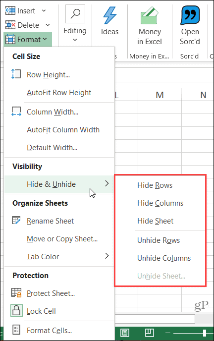

Once you hide single or multiple columns or rows, you’ll see a small indicator next to the surrounding columns or rows.


To quickly unhide columns or rows, right-click the indicator described above and click Unhide in the menu. Like with hiding them, you can also go to the Home tab, click Format, and select an Unhide option in the pop-out menu.
Group and Ungroup Columns and Rows
One more handy way to manage columns and rows are to group them. This is convenient if you have a subsection of items. For example, you may have a product sheet with sizes for an item. You can group these sizes together which you can then expand and collapse.
Select the columns or rows you want to group. You can do this by dragging through their headers or by clicking the first, holding your Shift key, and clicking the last.
Go to the Data tab and click the Group button which is in the Outline section on the right of the ribbon.


Once you group columns or rows, you’ll see a gray strip appear on the top for columns and side for rows. Within that strip is a line with a minus sign. The line represents the columns or rows in the group. Click the minus sign to collapse the group. Then, click the plus sign to expand it again.
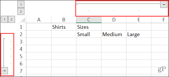

Another fast way to expand and collapse a group is with the numbered buttons that appear in the corner of that strip. You should see buttons labeled 1 and 2. Click the 1 button to collapse the group and the 2 button to expand it.


To ungroup columns or rows, head to the Data tab and click the Ungroup button.
View Your Excel Data Easier by Managing Columns and Rows
By freezing, hiding, or grouping columns and rows in Microsoft Excel, you have more ways to view your data. And when it comes to data entry, any way that you can make things quicker and easier is a blessing.
If you also work with spreadsheets in Google Sheets, check out our tutorial for freezing, hiding, and grouping columns and rows in Sheets too.
Stay up to date on our new articles by following us on Twitter or liking us on Facebook!


