How to Highlight Duplicates in Google Sheets

If you need to highlight duplicates in Google Sheets, you can use conditional formatting. Here’s how.
While Google Sheets doesn’t have the same depth of features as Microsoft Excel, it still has several useful tricks under the hood. One of its most useful features is conditional formatting.
This allows you to change the formatting of any cells that obey a specific set of conditions that you create. You could, for instance, highlight all of the cells that are above a certain value or contain a specific word. Conditional formatting has many uses, such as highlighting errors or comparing data.
Another useful application of conditional formatting is highlighting duplicates. This allows you to quickly spot any duplicate text or values within a large spreadsheet. Here’s how it’s done.
Highlighting Duplicates From a Single Column
If you want to highlight duplicates from a single column in Google Sheets, you’ll need first to select the column where you want to find duplicates.


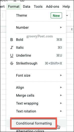
With your column selected, click Format > Conditional Formatting from the menu bar.

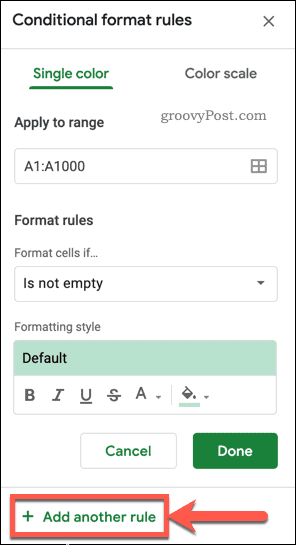
If you already have conditional formatting active in that column, click Add another rule. Otherwise, you can edit the rule that is currently showing.

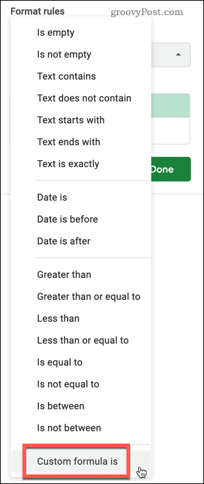
Press the Format Cells If box and choose Custom formula is from the dropdown options.

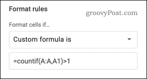
Type =countif(A:A,A1)>1 into the Value or formula box or replace all instances of the letter A in the formula with your chosen column.
For example, to apply the formatting to column M, your formula would be =countif(M:M,M1)>1

You can set the formatting style yourself by selecting the color and font options. You can also use one of the various preset formatting styles by clicking on the Default text under the Formatting style options, then selecting one of the presets.
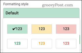

Click Done to add your conditional formatting rule. Any duplicate cells should now appear with your chosen highlighting.
Highlighting Duplicates From Multiple Columns
It’s possible to apply this formatting to more than one column, highlighting any duplicates that appear across your selected cell range.
To begin, select the columns that you want to include, hold down the Ctrl key, then click on the letter at the top of each column to add individual columns.
You can also hold down the Shift key and click on the first and last cells in your range to select multiple columns at once.


With your cells selected, press Format > Conditional Formatting.


Edit the current rule or press Add another rule to add a new rule.


Press the Format Cells If… option and choose Custom formula is.


Type =COUNTIFS($A$1:Z,A1)>1 into the Value or formula box. Replace each A with the letter of the first column in your selection and Z with the last column in your selection.
For example, if your data was in columns M to Q, then =COUNTIFS($M$1:Q,M1)>1 would be the correct formula.
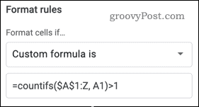

You can select your own formatting style in the Formatting style section or click on the Default text to apply one of several preset formatting options.


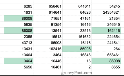
Click Done to confirm and save the rule—your duplicates will now be highlighted across all the columns you selected.
Any columns that you missed out on will not be highlighted but will still count towards duplicates.

Using Powerful Google Sheets Features
Conditional formatting is a useful feature that allows you to spot duplicated information across a large spreadsheet easily. Still, plenty of other features can be handy for Google Sheets beginners and regular users.
You may wish, for instance, to add in-cell validation to your spreadsheets to improve the quality of your data. If you’re looking to create automated tasks, you may want to look at using Google Sheets to send emails based on cell values.


